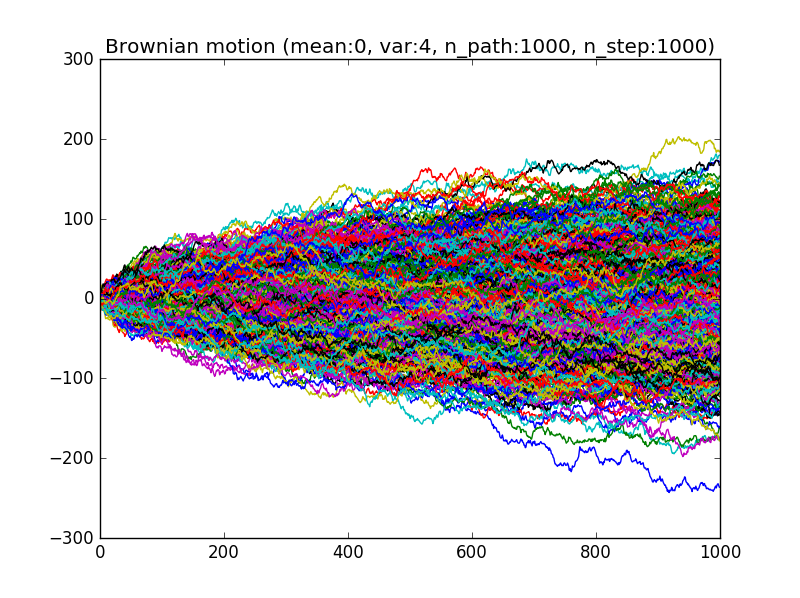
Brownian motion (布朗運動)

定義: Brownian motion

• A stochastic process $\{X(t), t \geq 0\}$ is said to be a Brownian motion process if
  • $X(0) = 0$.
  • $\{X(t), t \geq 0\}$ has independent increments $X(t)-X(s) \sim N(0, \sigma^2(t-s))$.
  • $\forall t >0, X(t) \sim N(0, \sigma^2 t)$.
  • $\forall t$, $X(t)$ is continuous.

• 由此可知，布朗運動每一點之間獨立。

• 若$\sigma = 1$，稱為標準布朗運動 (Standard Brownian motion)。

• 任何布朗運動，都可以藉由標準化$B(t) = \frac{X(t)}{t}$ 轉換為標準布朗運動。

定義 (in Shreve, Stochastic Calculus for finance)

• $(\Omega, F, P)$ is probability space.
• For each $\omega \in \Omega$, suppose there is a continuous function $W(t),\ t \geq 0$, which satisfies $W(0) = 0$ and depends on $\omega$.
• Then $W(t),\ t \geq 0$ is Brownian process if $\forall 0 = t_0 < t_1 < \cdots < t_n$, the increment $W(t_1)-W(t_0)$, $W(t_2)-W(t_1)$, \cdots $W(t_n) - W(t_{n-1}$ are mutual independent.
• Each of the increment is i.i.d. random variable of $N(0, t_{i+1} - t_{i})$
  • $E(W(t_{i+1}) - W(t_i)) = 0$.
  • $Var(W(t_{i+1}) - W_{t_i}) = t_{i+1} - t_i$.
  • $\therefore W(t) = W(t) - W(0) \sim N(0, t)$.

Filtration

• $(\Omega, F, P)$ is probability space, and Brownian process $W(t),\ t \geq 0$.
• A filtration for Brownian process is a collection of $\sigma$-field $F(t),\ t\geq 0$ satisfies:
  • Information accumulates (增大資訊集合), $0 \leq s \leq t$, $F(s) \subseteq F(t)$.
    • There is at least much information available at the later time $F(t)$ as there is at the earlier time $F(s)$.
    • 資訊為擴增的集合。
  • Adaptivity (適應性), $\forall t \geq 0$, $\lbrace w \vert W(t, \omega) \rbrace \in F(t)$ or called $W(t)$ is $F(t)$-measurable.
    • The information available at time $t$ is sufficient to evaluate the Brownian process $W(t)$ at this time.
    • 現在的事件必須可以用到目前為止的資訊集合評估。
  • Independence of future increment, $0 \leq s \leq t$, $P(W(t) - W(s) \vert F(s)) = P(W(t)-W(s))$.
    • Any increment of the Brownian process after time $t$ is independent of the information available at time $t$.
    • 未來的事件與現在的資訊集合獨立，即無法預測Brownian過程未來之值。
  • Properties (1) and (2) guarantee that the information available at teach time $t$ is at least as much as one would learn from observing the Brownian motion up to time $t$.

  ---

• There are two possibilities for the filtration $F(t)$ for Brownian process.
  • $F(t)$ contains only the information obtained by observing the Brownian process itself up time $t$.
  • If the information $F(t)$ includes observations of processes other than Brown process $W(t)$, this additional information is not allow to give clues about the future increments of $W$ because of the property (3).

Implementation

import numpy as np
import matplotlib.pyplot as plt

def brownian_motion(n_path, n_step=1000, mean=0, variance=1):
   points = np.random.randn(n_path, n_step)*np.sqrt(variance) + mean
   return(np.cumsum(points, axis=1))
n_path, n_step, mean, variance = 1000, 1000, 0 , 4
paths = brownian_motion(n_path, n_step, mean, variance)

for rdx in xrange(n_path):
 plt.plot(paths[rdx])

plt.title("Brownian motion (mean:{}, var:{}, n_path:{}, n_step:{})".format(
 mean, variance, n_path, n_step))

plt.show()

標準布朗運動性質

• $B(t) \sim N(0, t)$.

• $\{B(t), t\ \geq 0\}$ are a standard Brownian process,$0 < s < t, a,b \in \mathbb{R}$.

• $Cov(B(s), B(t))=E(B(s), B(t))=s,\forall s \leq t$.

  $\begin{array}{lcl} \because Cov(B(s), B(t)) & = & Cov(B(s), B(s)+B(t)-B(s)) \\ & = & Cov(B(s), B(s)) + Cov(B(s), B(t)-B(s)) [\text{indep. incr.}] \\ & = & Cov(B(s), B(s)) + 0 \\ & = & s. \end{array}$

• $Var(B(s)-B(t))=t-s$, $Var(B(t))=t$.
• $Var(aB(s)+bB(t))=(a+b)^2s + b^2(t-s)$.

  $\begin{array}{lcl} \because Var(aB(s)+bB(t)) & = & Var(aB(s)+b(B(s)+B(t)-B(s))) \\ & = & Var((a+b)B(s) + b(B(t)-B(s))) \\ & = & Var((a+b)B(s)) + Var(b(B(t)-B(s)) [\text{indep. incr.}] \\ & = & (a+b)^2s + b^2(t-s). \end{array}$

• $aB(s) + bB(t) \sim$ normal distribution.
• Covariance matrix of $(W(t_1), W(t_2), \cdots, W(t_n))$ is $\begin{bmatrix} E(W^2(t_1)) & \cdots & E(W(t_1) W(t_n)) \\ \vdots & \ddots & \vdots \\ E(W(t_n) W(t_1)) & \cdots & E(W^2(t_n)) \end{bmatrix}$

The density function

• $f_t(x) = \frac{1}{\sqrt{2\pi t}} e^{-\frac{x^2}{2t}}$.

The joint pdf

$\begin{array}{rcl} f(x_1,x_2, \cdots, x_n) & = & f_{t_1}(x_1) f_{t_2}(x_2 - x_1) \cdots f_{t_n - t_{n-1}} (x_n - x_{n-1}) \\ & = & \frac{1}{(2\pi)^{n/2}[t_1 (t_2-t_1) \cdots (t_n - t_{n-1})]^{1/2}}\exp\lbrace {-\frac{1}{2}\left[ \frac{x_1^2}{t_1} + \frac{(x_2 - x_1)^2}{t_2 - t_1} + \cdots + \frac{(x_n - x_{n-1})^2}{t_n - t_{n-1}}\right] }\rbrace \end{array}$

Conditional distribution

• Given $s < t$ and $B(t) = b$.

  • $f_{s\vert t} (x \vert b) = \frac{f_{s,t}(B(s)=x, B(t)=b)}{f_t(B(t) = b)} = \frac{f_s(x) f_{t-s}(b-x)}{f_t(b)} (\because \text{indep. incr.})$.

  • $\because f_s(x) = \frac{1}{\sqrt{2\pi s}} e^{-\frac{x^2}{2s}}$, $f_t(b) = \frac{1}{\sqrt{2 \pi t}}e^{- \frac{b^2}{2t}}$, and $f_{t-s}(b-x) = \frac{1}{\sqrt{2\pi (t-s}}e^{-\frac{(b-x)^2}{2(t-s}}$.

  • $\therefore f_{s \vert t} (x \vert b) = \frac{1}{\sqrt{2 \pi \frac{s(t-s)}{t}}} \exp {-\frac{(x-\frac{s}{t}b)^2}{2(\frac{s}{t}(t-s))}}$.

• $E(B(s) \vert B(t) = b) = \frac{s}{t}b$.

• $Var(B(s) \vert B(t) = b) = \frac{s}{t} (t-s)$.

Covariance

• $X(t), \ t \geq 0$ is Brownian process, $X(t) \sim N(0, \sigma^2 t)$.

• $0 < s < t$, $Cov(X(s), X(t) = \sigma^2 s$.

$\begin{array}{rcl} Cov(X(s), X(t)) & = & E(X(s) X(t)) \\ & = & E(X(s)(X(s) + X(t) - X(s))) \\ & = & Var(X(s)) + Cov(X(s), X(t) - X(s)) \\ & = & Var(X(s)) \\ & = & \sigma^2 s. \end{array}$

• Generally, $Cov(X(s), X(t)) = \lbrace \begin{array}{cl} \sigma^2 \min(\vert s \vert, \vert t \vert) & st > 0, \\ 0 & st < 0. \end{array}$

Correlation

• $Corr(X(s), X(t)) = \sqrt{\frac{t}{s}}$, $0 < s < t$.

$\begin{array}{rcl} Corr(X(s), X(t)) & = & \frac{Cov(X(s), X(t))}{\sqrt{Var(X(s)) Var(X(t))}} \\ & = & \frac{\sigma^2 s}{\sqrt{\sigma^2 s \sigma^2 t}} \\ & = & \sqrt{\frac{t}{s}}. \end{array}$

平賭(鞅)(Martingle process)

• $(\Omega, F, F_n, P)$ be a probability space, and $F_n$ is a flitration.

  • If $X(t) \in F_t$-measurable, $E(\vert X(t) \vert) < \infty$, and
  • $X(t) = E(X(t+1) \vert F_t)$.
  • then $X$ is a martingale process.

• $X(t)$ is a Brownian process, $X(t) \sim N(0, \sigma^2 t)$, the following are martingale processes:

  • $X(t)$
  • $X^2(t) - \sigma^2 t$
  • (Exponential martingale process) $\exp\lbrace \mu X(t) - \frac{\mu^2}{2} \sigma^2 t \rbrace,\ \mu \in \mathbb{R}$.

• $X(t)$ is martingale process.

  • $0 < s < t$, $X(t) = X(t) - X(s) + X(s)$.

    $\begin{array}{rcl} E(X(t) \vert F(s)) & = & E(X(t) - X(s) +X(s) \vert F(s)) \\ & = & E(X(t) - X(s) \vert F(s)) + E(X(s) \vert F(s)) \\ (\because X(t)-X(s) \text{ indep. to } F_s) & = & E(X(t) - X(s)) + X(s) \\ & = & X(s). \end{array}$

• $X^2(t) - \sigma^2 t$ is martingale process.

  $\begin{array}{rcl} X^2(t) & = & (X(t) - X(s) + X(s))^2 \\ & = & (X(t) - X(s))^2 + 2X(s)(X(t) - X(s)) + X^2(s) \end{array}$

  • $E((X(t) - X(s))^2 \vert F_s) = E((X(t) - X(s))^2) = (t-s)\sigma^2$.

  • $E(X^2(s) \vert F_s)=X^2(s)$.

  • $\therefore E(X^2(t) - \sigma^2 t \vert F_s) = (t-s)\sigma^2 + X^2(s) - \sigma^2 t = X^2(s) - \sigma^2 s$.

• $\exp \lbrace \mu X(t) - \frac{\mu^2}{2} \sigma^2 t \rbrace,\ \mu \in \mathbb{R}$. is martingale process.

  • $\mu X(t) = \mu (X(t) - X(s)) + \mu X(s)$.
  • $E(\exp(\mu X(t)) \vert F_s) = \exp(\mu X(s)) \cdot E(\exp(\mu (X(t) - X(s))))$.

  • $\because \ X(t) - X(s) \sim N(0, (t-s)\sigma^2)$,

    • the mgf $E(\exp(\mu (X(t)- X(s))) = \exp \left( \frac{\mu^2}{2} (t-s)\sigma^2 \right)$.

    $\begin{array}{rcl} \therefore E \left( \exp(\mu X(t) - \frac{\mu^2}{2} \sigma^2 t) \vert F_s \right) & = & \exp \left( \mu X(s) + \frac{\mu^2}{2} (t-s) \sigma^2 - \frac{\mu^2}{2} \sigma^2 t \right) \\ & = & \exp \left( \mu X(s) - \frac{\mu^2}{2} \sigma^2 s \right). \end{array}$

Shift property

• $X(t),\ t \geq 0$ is Brownian motion, $X(t) \sim N(0, \sigma^2 t)$.

• $\Rightarrow$ $Y(t) = X(t+r) - X(r), \ \forall r \in \mathbb{R}$ is Brownian process.

  • $E(Y(t)) = E(X(t+r) - X(r)) = E(X(t+r)) - E(X(r)) = 0$.

  • $Cov(Y(t), Y(s)) = \sigma^2 \min (t,s)$.

    $\begin{array}{rcl} Cov(X(t), X(s)) & = & E(X(t) X(s)) \\ & = & E( (X(t+r)-X(r))(X(s+r) - X(r)) \\ & = & E(X(t+r)X(s+r)) - E(X(t+r)X(r)) - E(X(r)X(s+r)) + E(X^2(r)) \\ & = & \sigma^2 \min(t+r, s+r) - \sigma^2 r - \sigma^2 r + \sigma^2 \\ & = & \sigma^2 \min(t,s). \end{array}$

  • $Y(t)$ is normal distribution.

Scaling property

• $X(t),\ t \geq 0$ is Brownian motion, $X(t) \sim N(0, \sigma^2 t)$.

• $\Rightarrow$ $Y(t) = \frac{X(c^2 t)}{c}, \ \forall c > 0$ is Brownian process.
  • $E(Y(t)) = 0$.

  • $Cov(Y(t), Y(s)) = \sigma^2 \min(t,s)$.

    $\begin{array}{rcl} Cov(X(t), X(s) & = & c^{-2} E(X(c^2 t) (c^2 s)) \\ & = & \sigma^2 c^{-2} \min(c^2t, c^2 s) \\ & = & \sigma^2 \min (t,s). \end{array}$

    • $Y(t)$ is normal distribution.

Brownian motion with drift

• 前面討論的Brownian motion都是沒有趨勢，即$E(X(t)) = 0,\ \forall t$.

• $X(t), \ t \geq 0$ is Brownian process with drift coefficient $\mu$ and variance parameter $\sigma^2$ if

  • $X(0) = 0$.
  • $X(t), \ t \geq 0$ has stationary and independent increments. * $X(t) \sim N(\mu t, \sigma^2 t)$.

• 等價定義, $B(t),\ t \geq 0$ is standard Brownian process and $X(t) = \sigma B(t) + \mu t$.

Geometric Brownian proces

• $Y(t),\ t \geq 0$ is Brownian process, and $Y(t) \sim N(\mu t, \sigma^2 t)$.

• Defintion: Geometric Brownian motion

  • $X(t) = e^{Y(t)},\ t \geq 0$.
  • i.e. $\ln X(t) = Y(t) \sim N(\mu t, \sigma^2 t)$.

• $E(X(t) \vert X(u), 0 \leq u \leq s) = X(s)E(e^{Y(t)- Y(s)})$.

  $\begin{array}{rcl} E(X(t) \vert X(u), 0 \leq u \leq s) & = & E(e^{Y(t)} \vert X(u), 0 \leq u \leq s) \\ & = & E(e^{Y(t) - Y(s) + Y(s)} \vert X(u), 0 \leq u \leq s) \\ (\because \text{indep. incr.}) & = & e^{Y(s)} E(e^{Y(t) - Y(s)} \vert X(u), 0 \leq u \leq s) \\ & = & X(s)E(e^{Y(t)- Y(s)}). \end{array}$

Standard Brownian bridge process

• Standard Brownian bridge process為起點與終點在相同位置的隨機過程。

• $B(t),\ t \geq 0$ is standard Brownian process, $B(t) \sim N(0, t)$.

• Let $Y(t) = B(t) - t B(0)$, $0 \leq t \leq 1$.

  • Y(0) = B(0) - 0 B(1) = 0.
  • Y(1) = b(1) - B(1) = 0‧
  • Standard Brownian bridge from $Y(0)=0$ to $Y(1) = 0$.

Standard Brownian bridge process properties

• $E(Y(t)) = E(B(t) - tB(0)) = 0$.

• $Cov(Y(t), Y(s)) = s(1-t)$, $0 < s < t < 1$.

  $\begin{array}{rcl} Cov(Y(t), Y(s)) & = & Cov(B(t) - tB(1), B(s) - sB(1)) \\ & = & Cov(B(t), B(s)) - s Cov(B(1), B(t)) - t Cov(B(s), B(1)) + st Cov(B(1), B(1)) \\ & = & s - st - st + st \\ & = & s(1-t). \end{array}$

Brownian bridge process

• $B(t),\ t \geq 0$ is standard Brownian process, $B(t) \sim N(0, t)$.

• Process start from $a$ at time $t=0$, achieve to $b$ at $t = T$.

* $Y(t) = a \left( 1-\frac{t}{T} \right) + b\frac{t}{T} + \left( B(t) - \frac{t}{T} B(t) \right)$, $0 \leq t \leq T$.

* {% math %}Y(0) = a{% endmath %}.
* {% math %}Y(T) = b{% endmath %}.

• $E(Y(t)) = a \left( 1 - \frac{t}{T} \right) + b \frac{t}{T}$.

• $Var(Y(t)) = t \left( 1- \frac{t}{T} \right)$.

  $\begin{array}{rcl} Var(Y(t)) & = & E\left( B(t) - \frac{t}{T} B(t)\right)^2 \\ & = & E^2(B(t)) - \frac{2t}{T} E(B(t) B(T)) + \frac{t^2}{T^2} E^2(B(T)) \\ & = & y - \frac{2t^2}{T} + \frac{t^2}{T^2} T\\ & = & t \left( 1 - \frac{t}{T} \right). \end{array}$

First-order variation

• 
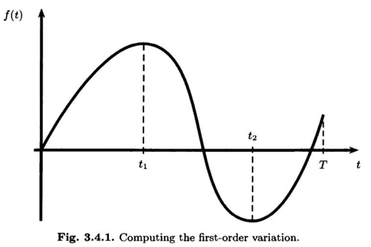
• 上圖中，依點$t_1$, $t_2$至$T$的函數變動量為$F_{V_T}(f) = (f(t_1) - f(t_0)) + (f(t_2) - f(t_1)) + (f(T) - f(t_2)) = \int_0^{t_1} f^{'}(t)dt + \int_{t_1}^{t_2} -f^{'}(t)dt + \int_{t_2}^T f^{'}(t)dt = \int_0^T \vert f^{'}(t) \vert dt$.
• Let partition $\pi =\lbrace t_0, t_1,\cdots, t_N \rbrace$ of $[0,T]$, and $\delta = \max_{0\leq k\leq N} (t_{k+1} - t_k)$.
• Define $F_{V_T}(f) = \lim_{\delta \rightarrow 0} \sum_{k=0}^{N-1}\begin{vmatrix} f(t_{k+1}) -f(t_k)) \end{vmatrix}$.
• By mean-value-theorem (MVT) of derivative
  • $\exists k \in t_k^{*} \in [t_k, t_{k+1}] \ni \frac{f(t_{k+1})-f_(t_k))}{t_{k+1}-t_k} = f^{(1)}(t_k^{*})$.
  • $\therefore f(t_{k+1} - f(t_k)) = f^{(1)}(t_k^{*}) (t_{k+1} - t_k)$.
  • $\sum_{k=0}^{N-1} f(t_{k+1}) - f(t_k) = \sum_{k=0}^{N-1} \begin{vmatrix} f^{(1)}(t_k^{*}) \end{vmatrix} (t_{k+1}) - t_k)$.
  • $\therefore \lim_{\delta \rightarrow 0} \sum_{k=0}^{N-1} \begin{vmatrix} f(t_{k+1}) - f(t_k)\end{vmatrix} = \lim_{\delta \rightarrow 0} \sum_{k=0}^{N-1} \begin{vmatrix} f^{(1)} t(_k^{*})\end{vmatrix} (t_{k+1} - t_k) = \int_0^T \begin{vmatrix} f^{(1)}(t_k^{*}) \end{vmatrix}dt$.
  • $\therefore F_{V_T}(f) = \int_0^T \begin{vmatrix} f^{(1)}(t_k^{*}) \end{vmatrix} dt$. (QED)

Quadratic variation

• The quadrativ variation of fucntion $f$ up to time $T$ is $[f,f](T) = \lim_{\delta \rightarrow 0} \sum_{k=0}^{N-1} (f(t_{k+1}) - f(t_k))^2$
• Suppose $f \in C^1([0,T])$ (i.e. $f$ has a continuous 1st derivative)

• $\sum_{k=0}^{N-1} (f(t_{k+1}) - f(t_k))^2 \leq \delta \sum_{k=0}^{N-1} \begin{vmatrix} f^{(1)}(t_k^{*})^2 \end{vmatrix}(t_{k+1} - t_k)$. $\begin{array}{rcl} [f,f](T) & \equiv & \lim_{\delta \rightarrow 0} \sum_{k=0}^{N-1} (f(t_{k+1}) - f(t_k))^2 \\ & \leq & \lim_{\delta \rightarrow 0} \left( \delta \sum_{k=0}^{N-1} \begin{vmatrix} f^{(1)}(t_k^{*})^2 \end{vmatrix}(t_{k+1} - t_k) \right) \\ & = & \lim_{\delta \rightarrow 0} \delta \lim_{\delta \rightarrow 0} \sum_{k=0}^{N-1} \begin{vmatrix} f^{(1)}(t_k^{*})^2 \end{vmatrix} (t_{k+1} - t_k) \\ & = & \lim_{\delta \rightarrow 0} \pi \int_0^T \begin{vmatrix} f^{(1)}(t)\end{vmatrix}^2 dt \end{array}$

• If $\lim_{\delta \rightarrow 0} \pi \int_0^T \begin{vmatrix} f^{(1)}(t)\end{vmatrix}^2 dt \leq \infty$ then $[f,f](T) = 0$.

• If $\lim_{\delta \rightarrow 0} \pi \int_0^T \begin{vmatrix} f^{(1)}(t)\end{vmatrix}^2 dt \rightarrow \infty$, then $[f,f](T)$ diverges.

• Brownian process is continuous, but not differentiabl everywhere, therefore the MVT is failed!!